In statistics, the most widely known and most frequently used distribution is probably the normal distribution (Gaussian distribution).
In bioscience and medical statistics as well, it is common practice to describe data using the expression
“mean ± standard deviation.” According to the central limit theorem, the sum of independent random variables
approaches a normal distribution regardless of the original form of the distribution. For example, it is known
that repeated convolution of a rectangular function converges to a Gaussian distribution in the limit.
Because of this powerful property, the normal distribution sometimes appears to be the “final form” of all distributions.
As a result, many studies have unconsciously adopted the approach of “assuming normality for the time being.”
However, when actual observational data are examined carefully, numerous distributions exhibit shapes
that differ significantly from the normal distribution. For instance, distributions that take only non-negative values,
peak near lower values, and possess a long decaying tail toward higher values are observed in biology, medicine, economics,
engineering, and many other fields. Such non-negative and right-skewed continuous distributions can be naturally described
by the gamma distribution from a statistical perspective.
From this viewpoint, the gamma distribution is often a more natural choice when describing non-negative continuous quantities.
Nevertheless, in both statistical education and practical applications, the normal distribution overwhelmingly dominates in
recognition and frequency of use, while the gamma distribution receives comparatively less attention.
Therefore, in this article, we aim to reexamine the properties and significance of the gamma distribution
in comparison with the normal distribution.
1. Historical Background
Behind the normal distribution and the gamma distribution stand two giants in the history of mathematics.
The normal distribution was systematized by the German mathematician Carl Friedrich Gauss (1777-1855)
in the context of analyzing astronomical observational errors. Introduced to explain variability in measurements,
it later became the standard “error distribution” and, through its connection with the central limit theorem,
established a position that appears almost universal in nature.
On the other hand, the “gamma function,” which forms the mathematical foundation of the gamma distribution,
was introduced in the 18th century by the Swiss mathematician Leonhard Euler (1707-1783).
The gamma function was originally developed as an extension of the factorial function—defined only for integers—into the realm of real numbers.
It was later applied to waiting-time distributions and stochastic processes, and was formalized as the gamma distribution in the late 19th century.

2. Comparison of Distribution Shapes
While textual explanations and mathematical expressions are important, differences between distributions are often more intuitively understood when visualized graphically. In particular, the contrast between the normal and gamma distributions becomes immediately apparent when their shapes are compared. Below are the probability density functions of both distributions.

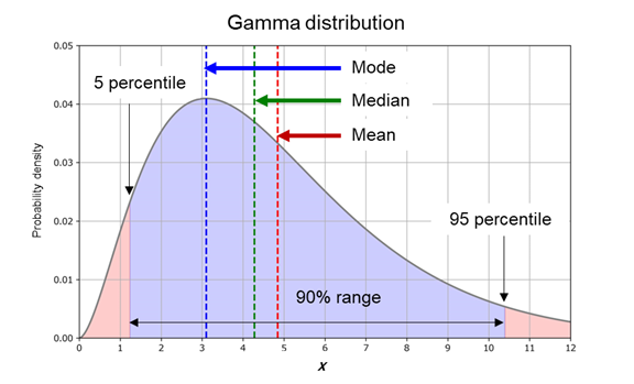
The symmetry of the normal distribution appears aesthetically pleasing.
In contrast, the asymmetric shape of the gamma distribution may initially feel somewhat unfamiliar.
For this reason, we may have unconsciously favored symmetry and accepted the normal distribution as the “standard form.”
As shown in the graph, in a Gaussian distribution the mean, median, and mode coincide exactly.
In a gamma distribution, however, these values generally differ, with mode < median < mean.
In the normal distribution figure, the range corresponding to one standard deviation is shaded.
The region “mean ± standard deviation” contains approximately 68.3% of the data.
Specifically, this corresponds to the 15.9th percentile and the 84.1st percentile.
An interesting question arises here: why do we habitually use this seemingly awkward 68.3% interval
instead of rounded values such as 5%, 95%, or 90% confidence intervals?
In fact, 68.3% has no special probabilistic significance.
It is merely a consequence that automatically arises from the mathematical parameter
called the standard deviation within the normal distribution formula.
The standard deviation determines the shape of the normal distribution mathematically,
and the ±σ interval emerges naturally from its internal structure.
Yet we routinely use this interval without consciously considering its mathematical origin.
2. Comparison of Distribution Functions
As shown in the previous section, the standard deviation \( \sigma \) is the mathematical parameter that determines the shape of the normal distribution, and its probability density function is expressed as follows:
For those who feel uneasy about mathematical formulas, this expression may appear complicated.
In reality, however, the normal distribution is completely determined by just two familiar parameters:
the mean \( \mu \) and the standard deviation \( \sigma \).
Similarly, the gamma distribution is also defined by two parameters:
the shape parameter \( \alpha \) and the scale parameter \( \beta \).
At first glance, this formula may appear even more complicated than that of the normal distribution.
In particular, the function \( \Gamma(\alpha) \) (the gamma function), as mentioned earlier,
was introduced by Euler as an extension of the factorial function into the real-number domain.
This structural complexity in the mathematical expression may be one reason why the gamma distribution
has not become as widespread as the normal distribution.
Furthermore, the shape parameter \( \alpha \) and the scale parameter \( \beta \) do not convey
an immediately intuitive meaning in the same way that the standard deviation \( \sigma \) does.
This lack of intuitive clarity may also have hindered the broader adoption of the gamma distribution.
However, in fact, \( \alpha \) and \( \beta \) can be determined from familiar descriptive statistics:
the mean and the mode. The mean of the gamma distribution is given by
\( mean = \alpha \beta \), and the mode is given by
\( mode = (\alpha - 1)\beta \).
In other words, once the peak of the distribution (the mode) and the mean are known,
the shape of the gamma distribution is uniquely determined.
Therefore, in general-purpose numerical tools such as spreadsheets, instead of directly entering
\( \alpha \) and \( \beta \), one could input the mean and the mode.
This approach may allow for more intuitive handling and could potentially broaden the practical use of the gamma distribution.
Even income distributions in everyday life exhibit a shape that peaks at lower values and
has a long decaying tail toward higher values. In such distributions, the mean may deviate significantly
from what most individuals actually experience, leading to the argument that
“the median better reflects reality.”
In the gamma distribution, the relationship between the mode and the mean itself determines the shape of the distribution.
Just as the expression “mean ± standard deviation” has become standard in the context of the normal distribution,
perhaps standardizing expressions such as “mode (mean)” in the context of the gamma distribution
could help us more naturally understand asymmetric distributions.
3. Versatility of the Gamma Distribution
In this section, we discuss the versatility of the gamma distribution by introducing several representative distributions.
3.1 The \( \chi^2 \) Distribution
In bioscience and medical research, the \( \chi^2 \) test is frequently used.
Its theoretical foundation is the \( \chi^2 \) distribution.
In fact, the \( \chi^2 \) distribution is nothing other than a special case of the gamma distribution.
If the degrees of freedom are denoted by \( k \),
then setting \( \alpha = k/2 \) and \( \beta = 2 \) in the gamma distribution
yields exactly the \( \chi^2 \) distribution.
An important point is that as the degrees of freedom \( k \) increase, the \( \chi^2 \) distribution gradually becomes more symmetric and approaches the normal distribution. This property follows from the central limit theorem. In the limit where the shape parameter \( \alpha \) becomes large, the gamma distribution asymptotically approaches the normal distribution. Therefore, the \( \chi^2 \) distribution can be regarded as a “special form” of the gamma distribution, while the normal distribution can be viewed as its “limiting form.”
3.2 Distribution of Anti-Müllerian Hormone (AMH) in Women of Reproductive Age
We hypothesized that the distribution of anti-Müllerian hormone (AMH)
in women of reproductive age follows a gamma distribution,
and we attempted mathematical modeling based on this assumption (see Reference).
It is well known that AMH levels decline with age as women approach menopause.
However, similar to income distributions, the distribution of AMH within a given age group
exhibits an asymmetric shape: a peak at lower values and a long tail toward higher values.
As a result, analyses based solely on the mean AMH value often created discrepancies
between statistical interpretation and patients' subjective perception of their own status.
Therefore, using data from approximately 7,000 individuals,
we performed a two-dimensional weighted nonlinear least squares regression
with the gamma distribution function as the model function
to mathematically model the AMH distribution.
The results for ages 27 to 45 are shown below.
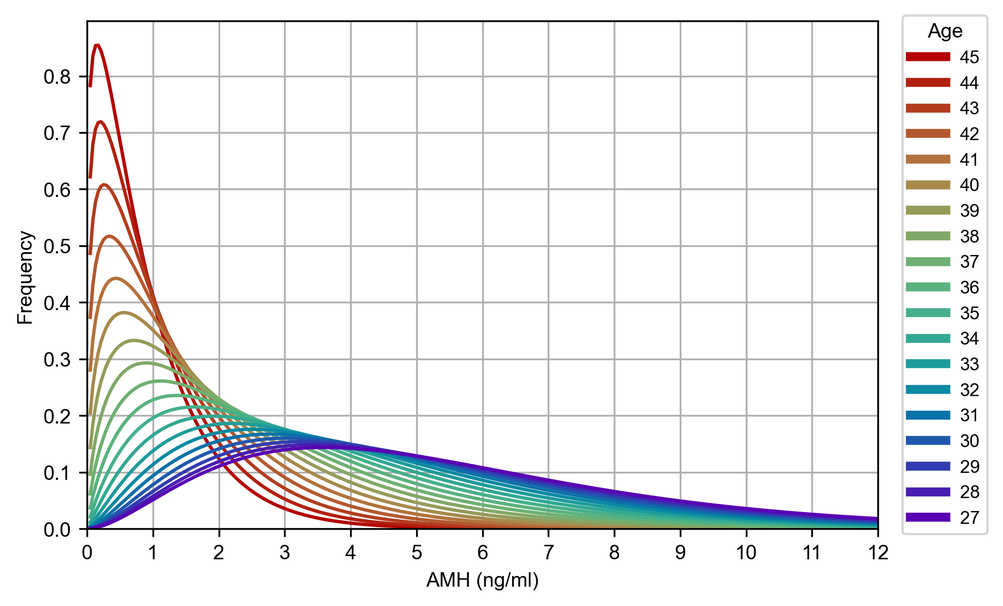
Whereas AMH distributions were traditionally expressed using the mean and standard deviation, applying the gamma distribution allows for a more accurate representation of the asymmetric structure observed in reality.
3.3 The First Electron Orbit of the Hydrogen Atom in the Bohr Model
Gerard 't Hooft, who received the Nobel Prize in Physics in 1999,
remarked regarding the foundations of quantum mechanics that
what is commonly called quantum mechanics today is essentially a probabilistic and statistical framework.
Although the examples discussed thus far have focused on medical applications,
it is fascinating that medicine, which routinely employs statistical analysis,
and theoretical physics, which deals with the microscopic world,
are connected through the shared language of probability and distributions.
In 1913, Niels Bohr proposed the hydrogen atom model
and theoretically derived the radius of the first electron orbit.
This achievement revolutionized our understanding of atomic structure,
and he received the Nobel Prize in Physics in 1922.
Bohr assumed that the electron moves in a circular orbit around the nucleus,
balancing Coulomb force with centripetal force, and imposed the quantization condition of angular momentum:
Using this relation, he derived the radius of the first orbit (\( n = 1 \)), which is given by:
This quantity is known as the Bohr radius.
However, in 1926, Max Born proposed that the position of the electron
in the hydrogen atom can only be described probabilistically until observed.
That is, it is not the wave function itself but its squared magnitude
\( |\psi|^2 \) that represents the probability density.
This probabilistic interpretation became foundational to quantum mechanics,
though Albert Einstein famously objected, stating, “God does not play dice.”
Thus began a major debate about the fundamental nature of quantum mechanics.
The wave function for the first orbit (ground state) of the hydrogen atom
is obtained by solving the Schrödinger equation.
For the state corresponding to principal quantum number \( n = 1 \)
and angular momentum quantum number \( l = 0 \),
the wave function is given by:
Here, \( r_B \) denotes the Bohr radius. Although the wave function itself is not directly observable, its squared magnitude
gives the probability density that the electron exists at distance \( r \). Considering that space is three-dimensional, the actual probability distribution for the electron being at distance \( r \) is obtained by multiplying by the volume element \( 4\pi r^2 \, dr \):
This expression exactly coincides with a gamma distribution when \( \alpha = 3 \) and \( \beta = r_B/2 \).
In other words, even the probability distribution describing the electron
in the hydrogen atom follows a gamma-type function.
Importantly, the Bohr radius \( r_B \) coincides with the peak of this distribution,
that is, the mode of the gamma distribution.
Meanwhile, the mean of this distribution is \( (3/2) r_B \),
which is larger than the mode.
The graph of this probability distribution is shown below.
Thus, although the most probable distance of the electron is \( r_B \),
the mean value lies farther outward.
This is due to the asymmetric shape with a long tail toward larger values.
This fact suggests that when a probability distribution is gamma-shaped,
the mode may serve as a more intuitive and physically meaningful representative value than the mean.
Afterword
In this article, we have explored the connection between medicine and physics
through the lens of the gamma distribution.
If quantum mechanics is fundamentally a probabilistic and statistical framework,
might similar quantum-mechanical analogies apply to probabilistic phenomena
such as live birth rates and AMH distributions in reproductive medicine?
In fact, my wife and I were blessed with our second child through assisted reproductive technology.
As someone whose profession involves statistical analysis,
I was told by my wife, “I don't believe in statistics. If I have a child, it's 100%; if I don't, it's 0%.”
A possibility that once existed as a probability distribution
collapses to either 100% or 0% the moment it is observed.
The same applies to the AMH distribution described above.
Initially, it exists as a probability distribution,
but at the moment a measurement is obtained,
it collapses to a single measured value.
Mathematically, this behavior resembles that of a delta function.
Repeating measurements reconstructs the original gamma distribution.
This structure may be analogously understood
as resembling the collapse of the wave function in quantum mechanics.
In quantum mechanics, we are often told that
“extraordinary phenomena beyond common sense occur in the microscopic world.”
However, even in the macroscopic world of human society,
might fundamentally similar structures exist?
Statistics itself may be a framework with dual characteristics:
governed by probabilistic laws as a whole,
yet containing randomness and free diversity in individual events.
Reference
Note: This page provides a summary as an introduction to the theory. For detailed mathematical models and statistical analysis methods, please refer to the publications below.